Statistical Error Reduction for Monte Carlo Rendering
Hiroyuki Sakai, Christian Freude, Michael Wimmer, David Hahn
Introduction
Ray tracing is a fundamental algorithm for producing photorealistic renderings that captures complex lighting phenomena such as shadows, reflections, and global illumination. To evaluate the rendering equation, Monte Carlo integration is used to stochastically sample light paths, and with finite samples comes unavoidable variance.
By using Monte Carlo integration to approximate the rendering equation, each pixel's color is estimated from a finite number of sampled light paths, and with finite samples comes variance. Formally, for a pixel with true radiance $\theta_j$, a path tracer produces a noisy estimate $\hat{\theta}_j$ whose sample variance $\hat{\sigma}^2_j$ decreases only as $1/n$ with the number of samples $n$. Achieving visually clean images therefore either demands an impractically large number of samples or a post-processing denoising step.
Denoising has become a standard part of ray tracing based rendering pipelines. Many approaches
today rely on neural networks. Systems like Intel Open Image Denoise
This report covers the implementation of the statistical denoising framework proposed by Sakai et al.
Previous Work
The problem of reducing noise in Monte Carlo rendered images has been a long-standing topic in Computer Graphics.
Classical approaches
use spatially adaptive filters—like Gaussian or bilateral—whose kernel widths are
guided by auxiliary information from the scene such as surface normals and albedos (collectively called G-buffers).
Rousselle et al. introduced adaptive sampling strategies driven by greedy MSE minimization
The shift toward neural methods began with the recurrent denoising autoencoder of Chaitanya et al.
The direct predecessor of the Sakai et al. paper is their own earlier work
Method
Unlike denoising methods that rely on machine learning, this framework uses statistical hypothesis testing to decide which neighboring pixels should be combined. This offers multiple advantages: no training data is required, the method is fully interpretable, and it provides theoretical convergence guarantees as sample count increases.
The core idea is to express denoising as a weighted average of neighboring pixel estimates. This is tantamount to defining a filter (such as a Gaussian filter) but intelligently selecting the weights to improve the image quality. For pixel $j$, the denoised estimate is:
$$\tilde{\theta}_j = \sum_i w_{ij} \hat{\theta}_i, \quad w_{ij} = \frac{\rho_{ij} m_{ij}}{\sum_i \rho_{ij} m_{ij}}$$
where $\rho_{ij}$ is a bilateral prior weight encoding distance in image, normal, and albedo space, and $m_{ij} \in \{0, 1\}$ is a statistical membership function that gates whether pixels $i$ and $j$ are compatible enough to be merged. For mean denoising, $m_{ij}$ is determined by Welch's t-test on the difference of pixel means:
$$m_{ij} = 1 \text{ if } |t| < t_{\nu, 1-\alpha/2}, \quad t=\frac{\hat{\theta}_i - \hat{\theta}_j}{\left(\hat{\sigma}^2_i/n_i + \hat{\sigma}^2_j/n_j\right)^{1/2}}$$
Multi-Transform Denoising
Monte Carlo sample distributions are typically non-normal due to the stochastic nature of light transport. Things like caustics, indirect illumination, and high-frequency materials all produce skewed distributions. Welch's t-test assumes normality, and its accuracy degrades under violations of this assumption. The Box-Cox power transformation can move a distribution closer to normality and is applied in this case to help normalize the distrubtions:
$$\ell^{(\lambda)}_{ik} = \begin{cases} (\ell^\lambda_{ik} - 1)/\lambda & \text{if } \lambda \neq 0 \\ \ln(\ell_{ik}) & \text{if } \lambda = 0 \end{cases}$$
Rather than using a single global transformation parameter, the method maintains statistics for multiple values of $\lambda$ simultaneously. This implementation, like the paper, uses $\lambda_1 = 0.25$ and $\lambda_2 = 1.0$ as the transformation parameters. The paper noted that 2 parameters was optimal. As the number of transformation parameters increases, so does the quality. However the return diminishes past 2 parameters, making the additional compute cost unjustifiable. For each pixel pair, the best transform is selected by minimizing the Jarque-Bera normality statistic:
$$\text{JB}^{(\lambda_m)}_{ij} = \text{JB}(\hat{\gamma}^{(\lambda_m)}_i, \hat{\beta}^{(\lambda_m)}_i, n_i) + \text{JB}(\hat{\gamma}^{(\lambda_m)}_j, \hat{\beta}^{(\lambda_m)}_j, n_j)$$
where $\hat{\gamma}$ and $\hat{\beta}$ are the sample skewness and kurtosis respectively. For mean denoising, the transform that maximizes the t-statistic (most discriminative) is selected. This empirically reduces overblurring at edges.
Linear Explained-Variance Correction
When a geometric edge crosses a pixel's footprint, the resulting sample distribution is multimodal—some samples hit the bright side, others the dark side—producing an inflated variance estimate. This overestimated variance can cause the denoiser to include too many neighbors, blurring the edge beyond what is desirable. The variance is decomposed using the law of total variance into an unexplained component (due to random sampling noise) and an explained component (due to the sub-pixel position of the sample):
$$\hat{\sigma}^2_\text{LEVC} = \hat{\sigma}^2 - c\,(|\text{Cov}(X, \mathbb{E}[L|X])| + |\text{Cov}(Y, \mathbb{E}[L|Y])|)$$
where $c = 4 \cdot \text{MAD}$ is a scaling factor based on the mean absolute deviation of the samples, and the covariances are estimated online during rendering using the sub-pixel coordinates of each sample.
Variance Denoising
One of the key innovations of the paper is applying the same statistical filtering framework to variance estimates themselves, not just pixel colors. Noisy variance estimates lead to poor membership decisions in the mean denoising step. By first denoising the variances, cleaner variance estimates are available for the subsequent mean denoising pass. The membership function for variance denoising tests whether the confidence interval for the variance ratio contains 1:
$$m_{ij} = 1 \text{ if } \hat{\sigma}^2_\Delta \leq \hat{se}_\Delta, \quad \hat{\sigma}^2_\Delta = |\ln(c_j \hat{\sigma}^2_j) - \ln(c_i \hat{\sigma}^2_i)|$$
Implementation
The full pipeline is implemented in WebGPU using WGSL compute shaders, running entirely on the GPU. The pipeline consists of three stages dispatched sequentially after path tracing completes: variance denoising (with LEVC applied first), mean denoising (using the denoised variances for cascaded denoising), and a final render pass that writes the denoised colors to the frame texture. Per-pixel statistics (the first four central moments, covariances, and MAD) are accumulated online during path tracing using Welford-style incremental updates. One set of statistics is maintained per Box-Cox transform parameter. The filter uses a 20-pixel radius bilateral base kernel weighted by image-space position, surface normal, and albedo.
Results
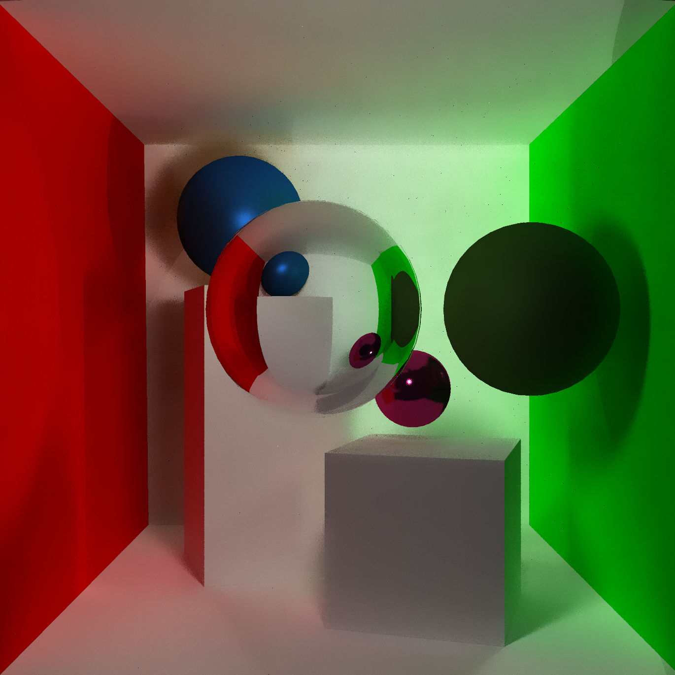
An interactive demo is available here. The demo provides an environment for exploring the denoising framework across three scenes: Cornell Box, Utah Teapot, and Fireplace Room. Note that the Fireplace Room is a large scene that may take significant time to load and render.
Upon selecting a scene, the path tracer runs first and the output image is progressively rendered tile by tile. Once complete, the denoising framework is applied. Variance and mean statistics are accumulated silently across the image before the final denoised result is displayed. A progress indicator tracks the overall render status. A toggle is also provided to disable denoising, making it easy to compare results directly.
The scene can be navigated using the mouse to rotate and the scroll wheel to zoom. Moving to a new viewpoint triggers the path tracer and denoiser to re-run on the updated configuration. Visible geometry can change significantly with viewing angle. This is particularly noticeable in the Fireplace Room. A material and lighting editor is also available via the side menu to futher modify and tune each environment.
Comparisons
The comparisons below show path-traced renders at 16 samples per pixel, before and after applying the statistical denoiser. Drag the slider to compare. The denoiser runs as a full-image post-process after all tiles have been rendered.
Flat surfaces such as walls and floors show the clearest improvement. Complex specular surfaces benefit from the variance denoising stage, which prevents overblurring near reflection boundaries. Some fine detail is lost in high-frequency regions. This is most visible in the carved woodwork on the walls of the Fireplace Room, where the denoiser over-smooths high-frequency texture.
Further experimentation is needed to evaluate performance across a broader range of scenes and sample counts. The hyperparameters used here follow those recommended in the paper, but initial investigation suggests they are somewhat scene-dependent. In particular, the significance level $\alpha$ and filter radius may benefit from per-scene tuning to better balance noise reduction against preservation of fine detail.
Cornell Box

.png)
Utah Teapot

.png)
Fireplace Room

.png)
Future Work
Several extensions would improve the quality and scope of the current implementation. A quick near-term improvement would be increasing the sample count per pixel. With only 16 samples, the statistical tests have very limited data and the denoiser must be conservative. Raising to 64 samples would significantly improve the reliability of the membership decisions and reduce residual noise on complex surfaces and would likely be necessary in a production environment.
Adaptive sampling, that is allocating more rays to high-variance pixels, is described in the paper as a first-class application of variance denoising but is not yet implemented here. This would provide a significant quality improvement for scenes with high variance variation, such as caustics or emissive geometry, without increasing the total ray budget.
The current filter uses MSE as its optimization target, which does not always align with perceptual quality. Incorporating a perceptual metric such as SSIM or LPIPS into the significance tests, as the paper suggests as future work, could reduce overblurring in textured regions while allowing more aggressive smoothing in perceptually flat areas.
Finally, exploring hybrid approaches that combine this statistical framework with machine learning would also be an interesting direction. Many existing nerual denoiser, rely solely on the albedo and normal information as auxiliary inputs. Providing the richer per-pixel statistically information generated with this method to a nueral network could provide a much richer signal that could potentially scale across larger varieties of scenes. This unlocks the way for exciting new research directions.
Bibliography
- H. Sakai, C. Freude, M. Wimmer, D. Hahn. Statistical Error Reduction for Monte Carlo Rendering. SIGGRAPH Asia, 2025.
- F. Rousselle, C. Knaus, M. Zwicker. Adaptive Sampling and Reconstruction using Greedy Error Minimization. ACM Trans. Graph., 2011.
- B. Moon, N. Carr, S. Yoon. Adaptive Rendering Based on Weighted Local Regression. ACM Trans. Graph., 2014.
- C. Schied et al. Spatiotemporal Variance-Guided Filtering: Real-Time Reconstruction for Path-Traced Global Illumination. HPG, 2017.
- M. Boughida, T. Boubekeur. Bayesian Collaborative Denoising for Monte Carlo Rendering. Comput. Graph. Forum, 2017.
- H. Sakai et al. A Statistical Approach to Monte Carlo Denoising. SIGGRAPH Asia, 2024.
- A. T. Áfra. Intel Open Image Denoise. https://www.openimagedenoise.org, 2025.
- C. R. A. Chaitanya, A. S. Kaplanyan, C. Schied, M. Salvi, A. Lefohn, D. Nowrouzezahrai, T. Aila. Interactive Reconstruction of Monte Carlo Image Sequences using a Recurrent Denoising Autoencoder. ACM Transactions on Graphics (SIGGRAPH), 36(4), 2017.